Plotting of Example Data
Imports
At first we need to point python to the project folder. The path can be assigned as a relative path as shown below, or as an absolute system path. For plotting of data the cloud_plotter modle is used, which can be imported via the import cloud_plotter command.
[1]:
import sys
from ctypytool import cloud_plotter

import warnings
warnings.filterwarnings("ignore")
Initialization
Our first step is to create a plotter object and to load a previously created cloud classifier project. Loading the project is neccesarry in order to import all project settings like the location of auxilary files.
[2]:
cp = cloud_plotter.cloud_plotter()

path = "../classifiers/ForestClassifier"
cp.load_project(path)
Next we specify some label files we want to plot. In this example the data consists of one original label file and two files of predicted labels, one from the Decision Tree and the other from the Random Forest Classifier.
[3]:
orig_file = "../data/example_data/nwcsaf_msevi-medi-20190317_1800.nc"
tree_prediction = "../classifiers/TreeClassifier/labels/nwcsaf_msevi-medi-20190317_1800_predicted.nc"
forest_prediction = "../classifiers/ForestClassifier/labels/nwcsaf_msevi-medi-20190317_1800_predicted.nc"
Plotting
Individual Plots
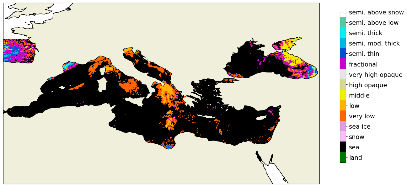
Using the plot_data method we can plot each of those datasets individually
[4]:
cp.plot_data(label_file = orig_file, colorbar = True)
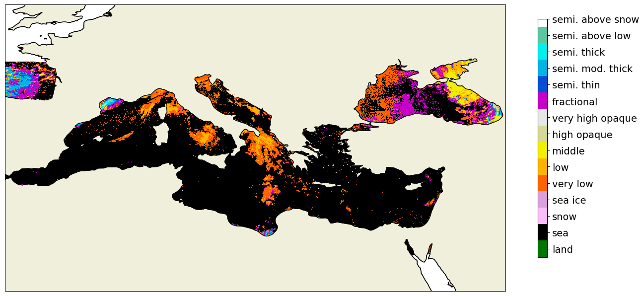
[5]:
cp.plot_data(label_file = tree_prediction, colorbar = True)
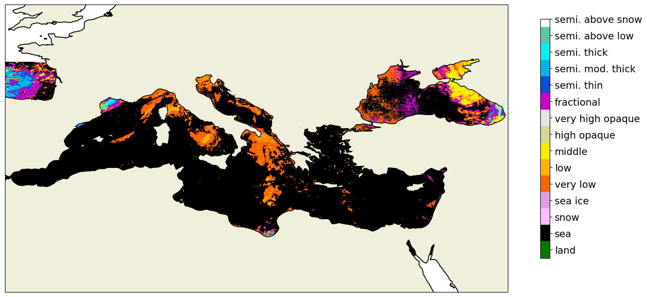
[6]:
cp.plot_data(label_file = forest_prediction, colorbar = True)
Combined Plots
Using the plot_multiple method we can plot multile datasets next to each other and evaluate the predcition performance in respect to the original labels.
[7]:
titles = ["Tree Classifier", "Forest Classifier"]
cp.plot_multiple(label_files = [tree_prediction, forest_prediction], truth_file = orig_file, plot_titles = titles)

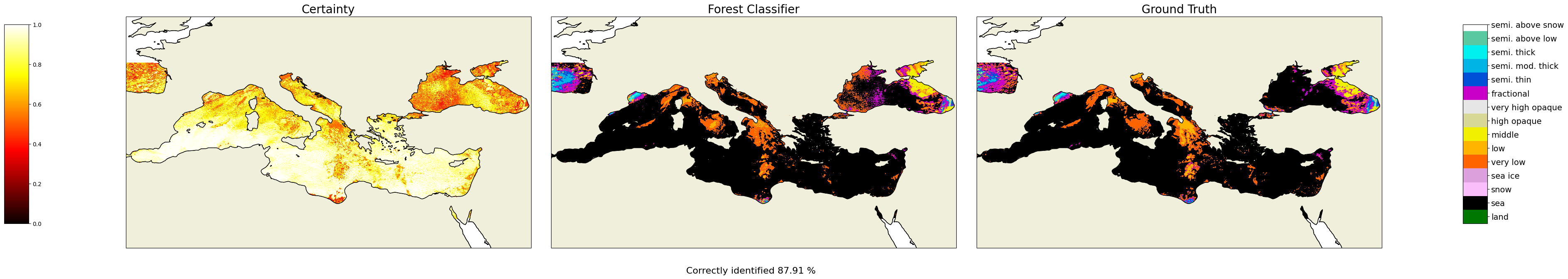
Probabilites Plots
The labels predicted with the Random Forest Classifier come with a probability score. That is, for each data point there also is a measure of how certain the classifier is about its choice of label. Those certainties are also stored in the label files and can be plooted using the plot_probas method.
[8]:
titles = ["Certainty", "Forest Classifier"]

cp.plot_probas(label_file = forest_prediction, truth_file = orig_file, plot_titles = titles)
Correlation Matrix Plots
Given predicted labels and the original file we can also compute and plot a correlation matrix via the plot_coocurrence_matrix method
[9]:
cp.plot_coocurrence_matrix(forest_prediction, orig_file)
